When Diversification Increases Risk

Intro

Harry Markowitz of Modern Portfolio Theory fame said that “Diversification is the only free lunch in investing” as it allows investors to reduce volatility without eroding returns. Diversification, through pooling of independent insured exposures, is also fundamental to risk management in insurance. But what if risk pooling actually increased risk?

The great Paul Embrechts and co-authors recently published an article entitled An unexpected stochastic dominance: Pareto distributions catastrophes, and risk exchange. In this brief post I will explore the paper’s unintuitive findings using simulation.

A brief review of the pareto distribution

The pareto distribution is a power-law distribution that was originally used to measure wealth inequality and underlies the familiar 80-20 rule. In its most basic form, it contains two variables, a shape variable $\alpha$, and a scale $\theta$ (minimum value, typically known) with probability density $f(x) = \frac{\alpha \theta^\alpha}{(x)^{\alpha + 1}}$, CDF $F(x) = 1 - (\frac{\theta}{x})^{\alpha}$ and mean $E[X] = \theta \frac{\alpha}{\alpha - 1}$.

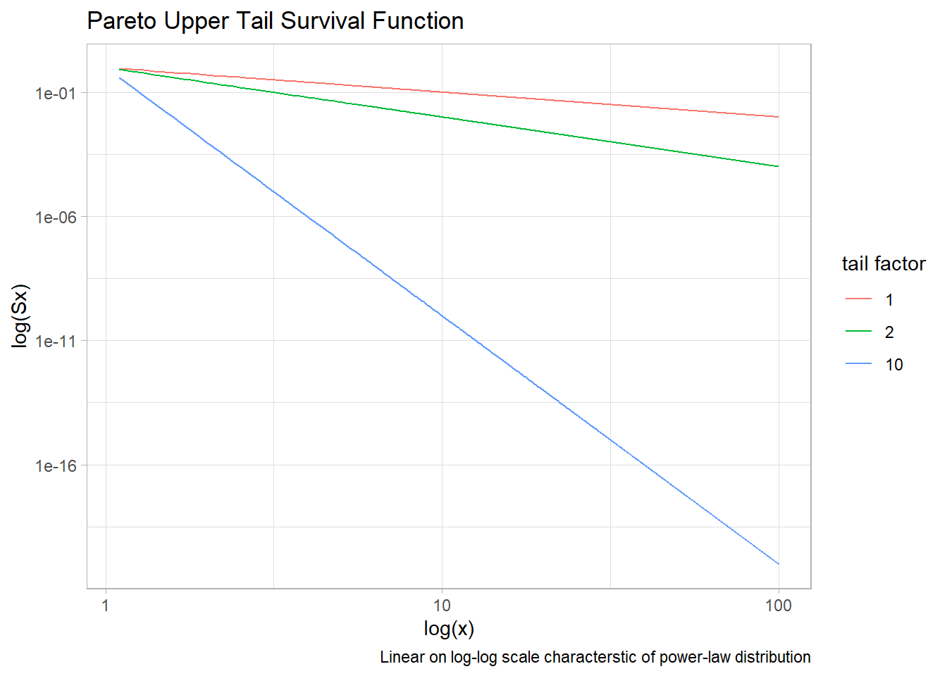
The shape $\alpha$, (“tail exponent”) controls the degree to which rare, extreme events disproportionately control the shape of the distribution (e.g.the mean).

Below you can see the effect of $\alpha$ on the tail of the distribution.

The unexpected stochastic dominance

Let’s first introduce the concept of stochastic dominance.

For two random variable X and Y representing random losses, we say X is smaller than Y in first-order stochastic dominance, denoted by $X \le_{st} Y$, if $P(X \le x) \ge P(Y \le x) for x \in \mathbb{R}$

This implies that X is the preferred risk for decision makers as globally, for a given loss amount x, it has a lower probability of exceeding x than Y.

The key result in the paper is Theorem 1.

For iid random variables $X_1, …, X_n$ following a Pareto distribution with infinite mean and weights $\theta_1, …, \theta_n$ with $\sum_{i = 1}^{n} \theta_i = 1$, our main finding in Theorem 1 is the stochastic dominance relation $$X_1 \le_{st} \theta_1 X_1 + … + \theta_n X_n$$

In plain english, for a pareto distributed variable with infinite mean (i.e.$\alpha < 1$), the quantiles (or Value at Risk–VaR) of a single random variable will be less than or equal to that of a “diversified” portfolio of identical risks!

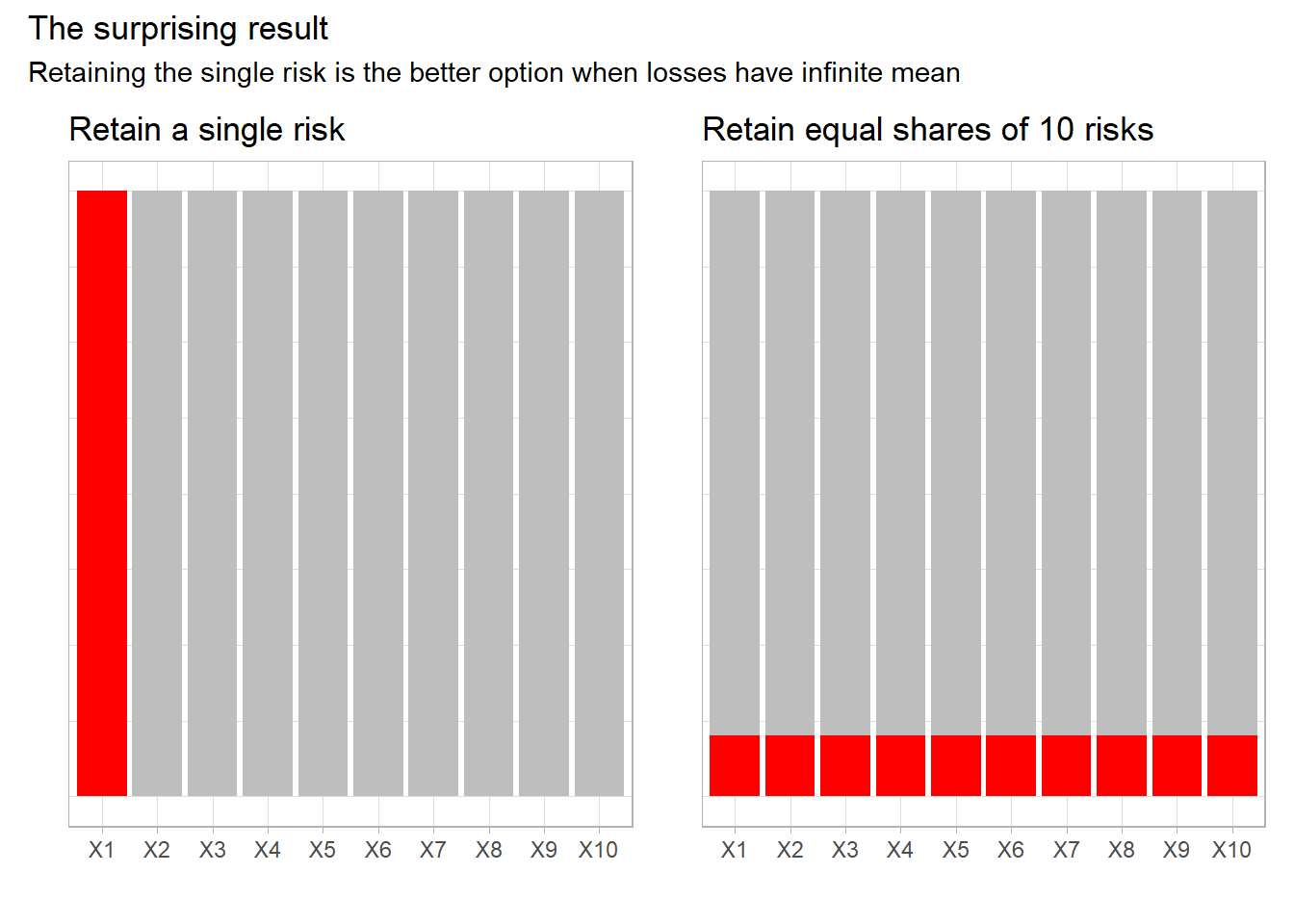
While VaR has been known to fail sub-additivity, that has been confined to some contrived cases and for select percentiles. The amazing result here is that this holds across the full distribution. You’re better off putting all your eggs in one basket!

A simulation approach

I’ll explore the finding above using simulation and visualization. I’ll utilize the *pareto functions from the EnvStats package.

Finite Mean

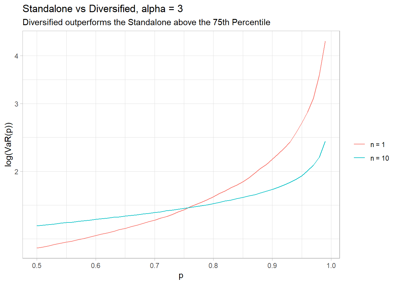
First lets look at the case of finite mean, where diversification works. We’ll simulate 10 iid parteo random variables with $\alpha = 3$ and compare the distributions of a standalone portfolio of X1 to a portfolio with 10 equal shares of X1:X10 $\frac{1}{n}\sum_{i = 1}^{n} X_i$.

To simulate I’ll write a function rpareto_n that, in addition to the tail factor, takes the number of risks n as an input and returns the average for each trial.

rpareto_n <- function(n = 1, alpha = 3, scale = 1, trials = 10e3){

  # Simulate n iid pareto variables
  sim <- matrix(rpareto(n * trials, shape = alpha, location = scale),
             nrow = trials)

  # equal proportions
  b <- rowSums(sim / n)

  return(b)

}

…and simulate.

sim_n1 <- rpareto_n(1, 3)
sim_n10 <- rpareto_n(10, 3)

Both distributions have the same mean (except for simulation error). But the diversified risk is the preferred one for the tail region (upper quartile). This is consistent with our intuition of the benefits of diversification.

Infinite Mean

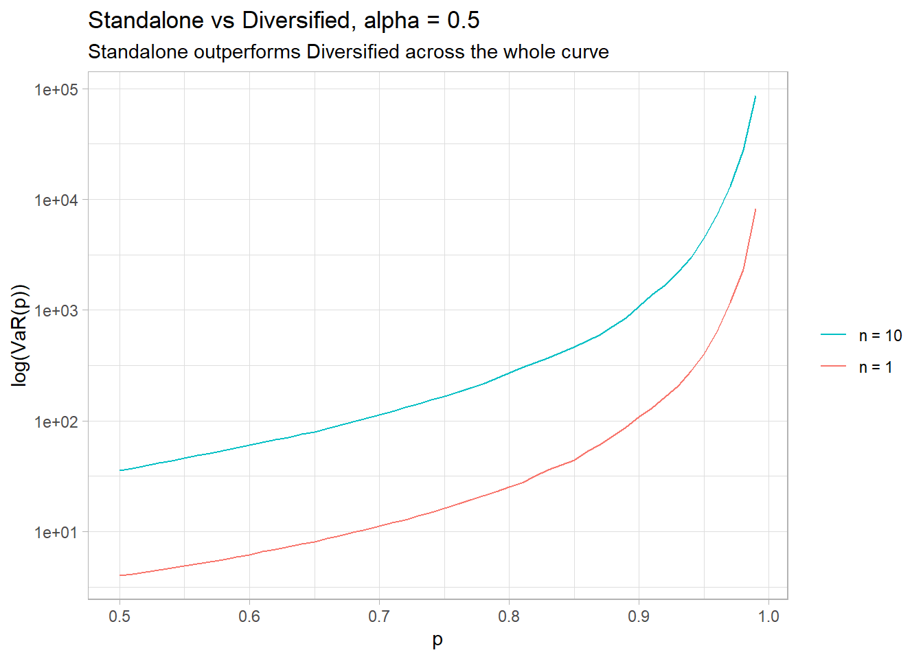
Now lets look at the same metrics using an infinite mean pareto, with $\alpha = 0.5$

The standalone risk now outperforms across the whole distribution!

Impact of Changing n

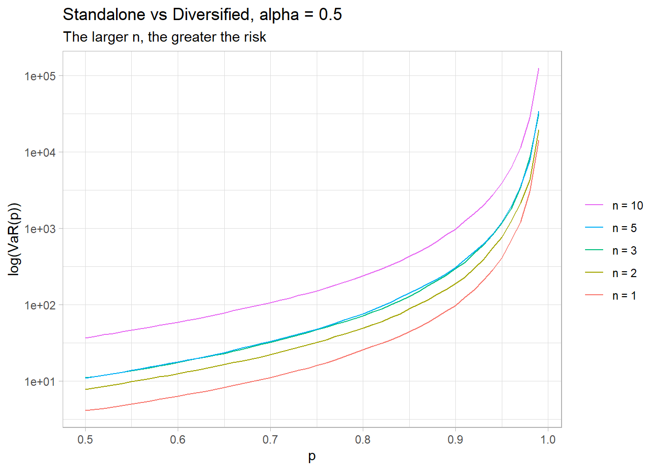
So we’ve seen that in an infinite mean regime, diversification failed with n=10 was worse than n=1. But what about n = 2, 3…?

Below I’ve repeated the simulation for additional number of risks.

When dealing with infinte mean random variables, the more “diversified” the exposure, the greater the risk!

Conclusion

While the result is amazing, we must consider that it’s limited to infinite mean distributions. The authors described some real world risks that had approximates tail factors of less than 1 (marine, wildfire losses). Certainly in the world of insurance where policy limits are the norm, we’d expect losses, no matter how extreme, to be bounded. That said, it’s a fascinating result with consequences for the future of risk management.

Note: Most code has been omitted for brevity. Source code here